Product Descriptions
There are several types of products that are provided through ManUniCast. These fall in 4 differing categories: maps (both 2D and 3D), cross sections (both west to east and south to north), Skew-Ts, and meteograms. The description for these differing types of maps follow.
Many of these descriptions and definitions originate from the American Meteorological Society Glossary of Meteorology, which is located at this address: http://glossary.ametsoc.org/wiki/.
Weather Products
2D Map
These maps are only plotted on one level, or are associated with the values at the surface.
- Dewpoint:
- The dewpoint temperature (in degrees Celsius) at 2m above the surface.
- Level of Free Convection (LFC):
- The height (in metres) at which an air parcel will rise without any additional forcing. From the level of free convection until the level which an air parcel returns to the environmental temperature the atmosphere is in a state of latent instability. A lower LFC can potentially indicate a more unstable atmosphere.
- Lifting Condensation Level (LCL):
- The height (in metres) at which an air parcel that has been lifted at the dry adiabatic lapse rate from the surface becomes saturated. A lower LCL indicates a moister atmosphere that may be more convective.
- Maximum Convective Available Potential Energy (CAPE):
- Amount of energy (in joules per kilogram) that is available to a
rising air
parcel. High values of CAPE can indicate a very unstable
atmosphere. Typical values of CAPE in the United Kingdom for
convective storms are less then 1000 J/kg, but can climb to values
exceeding 3000 J/kg in the midwestern United States. CAPE can be
defined as:
$$\mathrm{CAPE} = \int_{p_{n}}^{p_{f}}(\alpha_{p} - \alpha_{e})dp$$where \(\alpha_{e}\)is the environmental specific volume profile, \(\alpha_{p}\)is the specific volume of a parcel moving upward moist-adiabatically from the level of free convection, \(p_{f}\)is the pressure at the level of free convection, and \(p_{n}\)is the pressure at the level of neutral buoyancy.
- Maximum Convective Inhibition (CIN):
- The amount of energy (in joules per kilogram) that is necessary to
lift an air parcel from the surface to the level of free convection
(LFC). Higher values of CIN indicate that convection may be
less likely to form without sufficient upwards lifting caused by
other atmospheric conditions. CIN can be defined as:
$$\mathrm{CIN} = -\int_{p_{i}}^{p_{f}}R_{d}(T_{vp} - T_{ve}) d \ln p$$where \(p_{i}\)is the pressure at the level at which the parcel originates, \(p_{f}\)is the pressure at the LFC, \(R_{d}\)is the specific gas constant for dry air, \(T_{vp}\)is the virtual temperature of the lifted parcel, and \(T_{ve}\)is the virtual temperature of the environment.
- Maximum Simulated Radar Reflectivity:
- A derived radar return (in dBZ) from the model microphysical information about cloud water and ice content. The simulated reflectivity is supposed to use the available information from the atmospheric model output to simulate what the return echoes would be for a United States WSR-88D Doppler radar, and the maximum simulated radar reflectivity is the highest value of that calculated radar return in a column of air.
- Mixing Ratio (2D):
- The ratio of the mass of water vapor in the atmosphere at that point to the mass of dry air. The 2D map gives the mixing ratio at 2 metres above the surface. Typically given in units of grams per kilogram (g/kg), or 1000 times the actual ratio.
- Planetary Boundary Layer Height:
- The height (in metres) of the atmospheric boundary layer, which forms the interface between the surface and the free atmosphere. A low boundary layer height can indicate an inversion in the atmosphere that prevents the air from mixing, therefore causing negative effects on air quality.
- Potential Vorticity at 320 K:
- Potential vorticity, in potential vorticity units (PVU, 1 PVU = 1.0 × 10⁻⁶ m2 s-1K kg-1) at the 320 K isotropic level.
- Precipitable Water:
- The amount of water vapor in a column of air if all of it was condensed into liquid and fell as precipitation. Typically given in values of either kg/m2 or mm.
- Radar-derived rain rate at 1 km AGL:
This uses the simulated reflectivity at 1 kilometer above ground level to solve for R from this equation:
$$Z = 200 R^{1.6}$$where \(Z\) is the radar reflectivity factor and \(R\) is the rain rate. This provides a field that can be compared easily to the radar rain rate composite found at the UK MetOffice (http://www.metoffice.gov.uk/public/weather/observations/?tab=map&map=Rainfall).
- Relative Humidity (2D):
- The ratio of the vapor pressure to the saturation vapor pressure for water. Typically given in values of percentage. The 2D map gives the mixing ratio at 2 metres above the surface.
- Sea Level Pressure:
- The atmospheric pressure at sea level (in hPa or mb). Since most station locations are at an elevation higher then sea level, the surface pressure at those station locations (or model grid points) are then reduced to what it would be if the model grid point was at sea level by assuming that the temperature at the model grid point would remain constant.
- Simulated reflectivity at 1 km AGL:
- A derived radar return (in dBZ) from the model microphysical information about cloud water and ice content. The simulated reflectivity is supposed to use the available information from the atmospheric model output to simulate what the return echoes would be for a United States WSR-88D Doppler radar. The 1 km AGL simulated reflectivity interpolates the reflectivity field to 1 kilometer above ground level.
- Snowfall depth (2D):
- Total snow depth from model initialisation through plotting time (in metres). Snow height is calculated in the Noah land surface model based upon the compaction of a snowpack under conditions of increasing snow density. A full description of this process can be found in Koren (1999). Initial snow depths come from the GFS initial fields.
Koren, V. and Coauthors, 1999: A parameterization of snowpack and frozen ground intended for NCEP weather and climate models. J. Geophys. Res: Atmos., 104(D16), 2156–2202, doi: 10.1029/1999JD900232
Article link: http://onlinelibrary.wiley.com/doi/10.1029/1999JD900232/full - Snowfall rate (2D):
- Hourly snowfall in millimetres of liquid water equivalent. This field is the sum of the liquid water equivalents of all mixed phase or ice phase precipitation predicted by the Thompson microphysical parameterisation.
- Temperature (2D):
- The temperature (degrees Celsius) at 2 metres above the surface.
- Total Accumulated Precipitation:
- Precipitation from model initialisation through plotting time (in millimetres).
- Wind Speed (2D):
- The wind speed (in metres per second) at 10 metres above the surface.
- Wind Vectors (2D):
- Wind barbs of the 10 metre wind speed and direction. The wind barb points in the direction that the wind is coming from. A half-barb on the end indicates a 5 m/s wind speed, with a full barb a 10 m/s wind speed and a pennant 50 m/s wind speed.
3D Maps
These maps are plotted at multiple pressure levels throughout the atmosphere. These are standard pressure levels used throughout meteorology and are at 1000, 925, 850, 700, 500, 300, 250, and 200 hPa.
- Absolute Vorticity:
-
The sum of the vorticity of the Earth (Coriolis parameter) and the relative vorticity. It is displayed in units of 10-5 s-1.
The relative vorticity can be defined as:
$$\zeta = \nabla \times \mathbf{u}$$where \(\zeta\) is the vorticity, \(\mathbf{u}\) the velocity, and \(\nabla\) the del operator.
The absolute vorticity can be represented by:
$$\eta = \zeta +f$$where \(\eta\) is the vertical component of the absolute vorticity vector, \(\zeta\) is the relative vorticity, and \(f\) is the Coriolis parameter.
Maxima in absolute vorticity indicate centers of rotation for large-scale weather systems within the atmosphere. Typically, absolute vorticity is viewed at 500 hPa in order to gauge the relative strength of the large-scale rotation of differing systems as well as the center of rotation in the middle of the atmosphere.
- Equivalent Potential Temperature:
- The temperature (in Kelvin) of an air parcel if it was brought down to the surface at the moist adiabatic lapse rate.
- Geopotential Height:
-
The height (in metres) of a given point in the atmosphere in units proportional to the potential energy of unit mass (geopotential) at this height relative to sea level.
The relation between the geopotential height \(Z\) and the geometric height \(z\) is
$$Z = \frac{1}{980}\int_{0}^{z}gd{z}'$$where \(g\) is the acceleration of gravity. The two heights can nearly be considered the same in most meteorological purposes.
- Layer Thickness from 1000 hPa:
- The thickness (in metres) of the geopotential height (see above) from 1000 hPa to the selected atmospheric level. The layer thickness gives an idea about the average column temperature. Low pressure centers due to their cold core structures will typically have a lower thickness then the surrounding atmosphere, although tropical storms have a warm core structure and therefore would higher thickness then the surrounding atmosphere.
- Mixing Ratio (3D):
- The ratio of the mass of water vapor in the atmosphere at that point to the mass of dry air. The 3D maps give the mixing ratio at the standard atmospheric levels. Typically given in units of grams per kilogram (g/kg), or 1000 times the actual ratio.
- Moist Potential Vorticity:
- Potential vorticity, in potential vorticity units (PVU, 1 PVU = 1.0 × 10⁻⁶ m2 s-1K kg-1) at various pressure levels throughout the atmosphere. Moist potential vorticity differs from potential vorticity due to use of equivalent potential temperature instead of potential temperature during its computation.
- Potential Temperature:
- The temperature of an air parcel (K) if it descended to the surface at the dry adiabatic lapse rate.
- Potential Vorticity:
- Potential vorticity, in potential vorticity units (PVU, 1 PVU = 1.0 × 10⁻⁶ m2 s-1K kg-1) at various pressure levels throughout the atmosphere.
- Relative Humidity (3D):
- The ratio of the vapor pressure to the saturation vapor pressure for water. Typically given in percentages (%). The 3D maps give the relative humidity at the defined pressure level.
- Temperature (3D):
- The temperature (in degrees Celsius) at the defined pressure level.
- Vertical Velocity:
- The wind speed (in metres per second) in the upwards (positive) or downwards (negative) directions at the defined pressure level.
- Wind Speed (3D):
- The wind speed (in metres per second) at the defined pressure level.
- Wind Vectors (3D):
- Wind barbs at the defined pressure level. The wind barb points in the direction that the wind is coming from. A half-barb on the end indicates a 5 m/s wind speed, with a full barb a 10 m/s wind speed and a pennant 50 m/s wind speed.
Cross Sections
These plots are vertical slices of the atmosphere, either along 2 degrees west longitude or 53 degrees north latitude. This is meant to show how the weather systems proceed across the UK and also how they change with height. It can also give an idea of the depth of differing circulations. Several of the fields are reproduced from either the 2D or 3D maps, and their descriptions are repeated here.
- Cloud Water Mixing Ratio:
- The ratio of the mass of condensed water in the air to the total mass of the air. Typically given in units of grams per kilogram (g/kg), or 1000 times the actual ratio.
- Cloud Ice Mixing Ratio:
- The ratio of the mass of condensed ice in the air to the total mass of the air. Typically given in units of grams per kilogram (g/kg), or 1000 times the actual ratio.
- Equivalent Potential Temperature:
- The temperature (in Kelvin) of an air parcel if it was brought down to the surface at the moist adiabatic lapse rate.
- Potential Temperature:
- The temperature of an air parcel (K) if it descended to the surface at the dry adiabatic lapse rate.
- Potential Vorticity:
- Potential vorticity, in potential vorticity units (PVU, 1 PVU = 1.0 × 10⁻⁶ m2 s-1K kg-1) at various pressure levels throughout the atmosphere.
- Relative Humidity:
- The ratio of the vapor pressure to the saturation vapor pressure for water. Typically given in values of percentage. The cross sections give a vertical profile of the moisture present in the atmosphere.
- Simulated Radar Reflectivity:
- A derived radar return (in dBZ) from the model microphysical information about cloud water and ice content. The simulated reflectivity is supposed to use the available information from the atmospheric model output to simulate what the return echoes would be for a United States WSR-88D Doppler radar.
- Temperature (Cross section):
- The temperature (in degrees Celsius) throughout the atmosphere.
- Vertical Velocity (Cross section):
- The wind speed (in metres per second) in the upwards (positive) or downwards (negative) directions.
- Wind Speed (Cross section):
- The wind speed (in metres per second) at the vertical cross section.
- Wind Vectors (Cross section):
- Arrows indicating the direction of the wind along the cross section.
- Wind Streamline (Cross section):
- Arrows indicating the trajectory of the wind along the cross section.
Skew-Ts and Meteograms
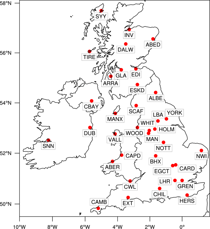
Both Skew-T's and meteograms are point measurements, and are representative of the points given on this map:
| Site ID | Site Name |
|---|---|
| ABED | Aberdeen, Scotland |
| ABER | Aberporth, Wales |
| ALBE | Albermare, Northumberland, England |
| ARRA | Isle of Arran, Scotland |
| BHX | Birmingham Airport (BHX), Scotland |
| CAMB | Camborne, Cornwall, England |
| CAPD | Capel Dewi, Wales |
| CARD | Cardington, Bedfordshire, England |
| CBAY | Castor Bay, Northern Ireland |
| CHIL | Chilbolton Observatory, Hampshire, England |
| CWL | Rhoose Cardiff-Wales Airport (CWL) |
| DALW | Dalwhinney, Inverness-shire, Scotland |
| DUB | Dublin Airport (DUB), Ireland |
| EDI | Edinburgh Airport (EDI), Scotland |
| EGCT | Cranfield Airport (EGCT), England |
| ESKD | Eskdalemuir, Scotland, Scotland |
| EXT | Exeter Airport (EXT), England |
| GLA | Glasgow Airport (GLA), Scotland |
| GREN | Royal Observatory, Greenwich, England |
| HERS | Herstmonceux, Sussex, England |
| HOLM | Holme Moss, West Yorkshire, England |
| INV | Inverness Airport (INV), Scotland |
| LBA | Leeds/Bradford Airport (LBA), England |
| LHR | London/Heathrow (LHR), England |
| MAN | Manchester Airport (MAN), England |
| MANX | Isle of Man |
| NOTT | Nottingham Weather Centre, England |
| NWI | Norwich Airport (NWI), England |
| SCAF | Scafell Pike, Cumbria, England |
| SNN | Shannon Airport (SNN), Ireland |
| SYY | Stornoway Airport (SYY), Scotland |
| TIRE | Tireee, Argyll, Scotland |
| VALL | Valley, Gwynedd, Wales |
| WHIT | Whitworth Observatory, Manchester, England |
| WOOD | Woodvale, Merseyside, England |
| YORK | York, England |
Skew-Ts
A Skew-T log-P chart is a diagram of a profile of the atmospheric temperature, dewpoint, and wind speed. It is used to examine the vertical structure of the atmosphere at that grid point as well as to determine the stability of the air at that point. A ManUniCast Skew-T gives several different forms of information at the top as well:
- PLCL - the pressure of the Lifting Condensation Level (hPa)
- TLCL - The temperature of the LCL (degrees C)
- Shox - Showalter Index, a stability index
- Pwat - The precipitable water in the column (cm)
- CAPE - the convectively available potential energy (J/kg).
Meteograms
Meteograms show 78-hour plots of relative humidity (%), temperature (C), precipitation (mm), surface pressure (hPa), wind speed (m/s), and wind direction (degrees). These are meant to show the diurnal patterns over the 78-hour forecast cycle and represent the surface weather at the model grid point that is closes to the given location (as represented by the map above).
Chemistry Products
2D & 3D Maps
- Gas-phase Chemical Mixing Ratios:
- For our atmospheric chemistry predictions (dchem) we plot mixing ratios of the following chemical compounds: ammonia (NH3), carbon monoxide (CO), dinitrogen pentoxide (N2O5), formaldehyde (HCHO), hydrogen peroxide (H2O2), nitrate radical (NO3), nitric oxide (NO), nitrogen dioxide (NO2), ozone (O3), peroxyacylnitrate (PAN), and sulpher dioxide (SO2). These mixing ratios are in parts per million by volume (ppmv), parts per billion by volume (ppbv) or parts per trillion by volume (pptv) (as denoted on the plots for each chemical compound). We also plot the mixing ratio of the sum of all non-methane volatile organic compounds (NM-VOC's) in ppbv, and the concentration of the hydroxyl radical (OH) in molecules per cubic centimetre of air.
- Particulate Matter (PM) Mass Loadings:
-
For our atmospheric chemistry predictions (dchem) we plot the mass loadings (in micrograms per cubic metre of air at standard atmospheric pressure) of a number of aerosol products. The MOSAIC aerosol scheme distributes the aerosol particles across 8 internally mixed size sections, covering the size range of 3 nanometre diameter up to 10 micrometre diameter particles. We have summed up these size bins to represent the composition of particulate matter of the size ranges: 10 micrometres or less diameter (PM10); 2.5 micrometres or less diameter (PM2.5); and 1 micrometre or less diameter (PM1). The first of these is the sum of all aerosol size sections, the second is the sum of the smallest 6 size sections, and the third is the sum of the smallest 4 size sections plus a fraction (0.678) of the 5th smallest size section.
The products we plot for PM10 aerosol are total mass loading, dust (OIN), and seasalt (sodium plus chloride). We also plot total aerosol number concentration (in particles per cubic metre of air at standard atmospheric pressure).
The products we plot for PM2.5 aerosol are total mass loading, ammonium, sulphate, nitrate, sodium, chloride, black carbon, and organic particulate matter.
The products we plot for PM1 aerosol are inorganic (the sum of ammonium, sulphate, nitrate, sodium and chloride), black carbon, and organic particulate matter.
- Cloud Condensation Nuclei Concentrations:
- These are the number concentrations (particles per cubic metre of air at standard atmospheric pressure) of aerosol particles which will act as condensation nuclei for the formation of cloud droplets at a given water vapour supersaturation (in this case 0.2%, 0.5%, and 1.0%).
Meteograms
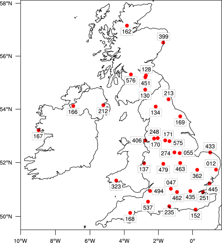
The meteograms are point measurements, and are representative of the points given on the following map. In addition, measurements for Dublin, London and Paris are also available.
| Site ID | Site Name |
|---|---|
| UKA00012 | Sibton |
| UKA00047 | Harwell |
| UKA00055 | Bottesford |
| UKA00128 | Bush Estate |
| UKA00130 | Eskdalemuir |
| UKA00134 | Great Dun Fell |
| UKA00137 | Aston Hill |
| UKA00152 | Lullington Heath |
| UKA00162 | Strathvaich |
| UKA00166 | Lough Navar |
| UKA00167 | Mace Head |
| UKA00168 | Yarner Wood |
| UKA00169 | High Muffles |
| UKA00170 | Glazebury |
| UKA00171 | Ladybower |
| UKA00212 | Belfast Centre |
| UKA00213 | Newcastle Centre |
| UKA00235 | Southampton Centre |
| UKA00248 | Manchester Piccadilly |
| UKA00251 | Rochester Stoke |
| UKA00274 | Nottingham Centre |
| UKA00323 | Narberth |
| UKA00362 | Wicken Fen |
| UKA00399 | Aberdeen |
| UKA00406 | Wirral Tranmere |
| UKA00433 | Weybourne |
| UKA00435 | London Westminster |
| UKA00445 | St Osyth |
| UKA00451 | Auchencorth Moss |
| UKA00462 | Reading New Town |
| UKA00463 | Market Harborough |
| UKA00479 | Birmingham Tyburn |
| UKA00486 | Lerwick |
| UKA00494 | Bristol St Paul's |
| UKA00537 | Charlton Mackrell |
| UKA00575 | Sheffield Devonshire Green |
| UKA00576 | Glasgow Townhead |
Meteogram Products
Meteograms show 54-hour plots of ozone (O3), nitric oxide (NO), nitrogen dioxide (NO2), sulphur dioxide (SO2), PM10 aerosol and PM2.5 aerosol. Also shown are plots of relative humidity (%), temperature (C), precipitation (mm), surface pressure (hPa), wind speed (m/s), and wind direction (degrees). These are meant to show the atmospheric chemistry predictions at the model grid point that is closest to the given location (as represented by the map above).